Molecular Energetics Group

Differential scanning calorimetry (DSC) is mainly used at the Molecular Energetic Group for the determination of temperatures and enthalpies of phase transitions (solid-liquid or solid-solid) and thermal decompositions (e.g. dehydrations), and heat capacities of solids and liquids.

Physical and chemical changes may often be induced by raising or lowering the temperature of a substance. Typical examples are phase transitions, such as fusion, or chemical reactions, such as the dehydration of a solid hydrate.

Differential scanning calorimetry (DSC) was designed to obtain the enthalpy and temperature of those processes, and also to measure temperature-dependent properties of substances, such as the heat capacity. This is done by monitoring the differential heat flow rate to a sample (S) and to reference cell (R):

as a function of time or temperature, while both S and R are subjected to a controlled temperature program. The temperature is usually increased or decreased linearly at a predetermined rate but isothermal experiments can also be performed. In some cases DSC experiments may provide kinetic data.

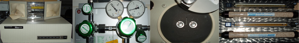
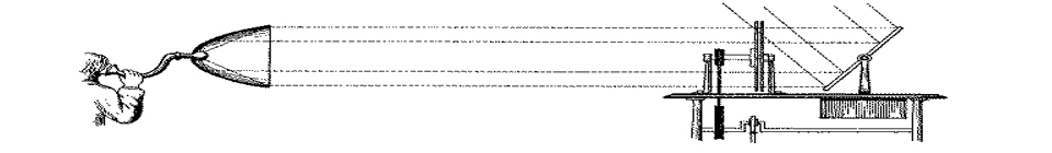
Two general types of DSC apparatus, which differ on the operation principle, are available: heat flux DSC and power compensation DSC. The equipment used at the Molecular Energetics group is a power compensation DSC 7 from Perkin Elmer (Figure 1).

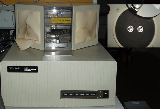
Figure 1. Power compensation DSC 7 from Perkin Elmer.

 

In a heat flux DSC, the temperature difference between the sample S and the reference R is recorded and converted to a difference in heat flow rate to the sample and to the reference, using a suitable calibration factor. In a power compensation DSC (Figure 2) the sample and the reference crucible holders consist of two small furnaces, 1_S and 1_R, each one equipped with a temperature sensor, 2_S or 2_R, and a heat source, 3_S or 3_R. The furnaces are located inside a cell 4 whose temperature is not monitored. The system of furnaces is controlled by two separate loops, one for average temperature control and the other for differential temperature control. The average temperature control loop ensures that the average of the sample and reference temperatures is increased at a programmed rate β. If the sample undergoes an endothermic or exothermic transformation, or a heat capacity change, a temperature difference, ΔT, will tend to develop between 1_S and 1_R. The differential control loop automatically adjusts the power supplied to each furnace, so that ΔT is maintained as close to zero as possible during an experiment (the value of ΔT is actually never zero because the working principle of the control system is based on the existence of a small error signal). The recorded output signal of the calorimeter is proportional to the differential heat flow rate, ΔΦ, between the sample and the reference. In the case of fusion, for example, the overall ΔΦ vs t difference will be detected as a peak in the measuring curve, whose onset gives the temperature of fusion of the sample and the area is proportional to the corresponding enthalpy of fusion.

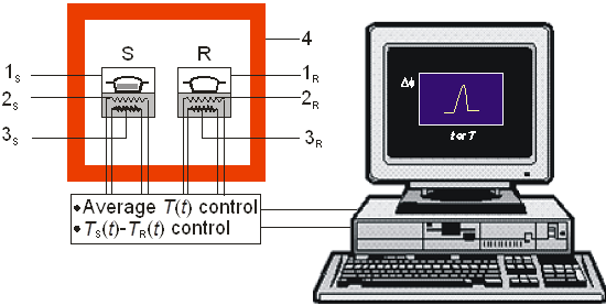
Figure 2. Calorimeter control circuits (see text for details).

 

The molar enthalpy of fusion, Δ_fusH_m , is calculated from:

(2)

where m and M are the mass and the molar mass of the sample, respectively, A is the area of the experimental curve, and ε is the energy equivalent of the calorimeter. The value of ε is obtained by calibration. The most widely recommended calibration method involves the determination of the enthalpy of fusion of one or more standard substances (e.g. indium). These studies also allow the calibration of the temperature scale of the instrument based on the observed temperature of fusion onsets.

The enthalpy of fusion given by equation (2) strictly refers to a non-isothermal process such as:

A(s, Ti) → A(l, Tf)

(3)

where Ti and Tf represent the initial and final temperature of the peak. Normally the difference Tf-Ti is not very large. In this case it is generally a good approximation to assume that the experimentally obtained Δ_fusH_m value refers to an isothermal process occurring at the onset temperature of the process. Nevertheless, the calculation of the enthalpy of the fusion process under isothermal conditions from Δ_fusH_m can be performed as described in reference [1].

The determination of the heat capacity as a function of the temperature usually involves three consecutive measurements (Figure 3).

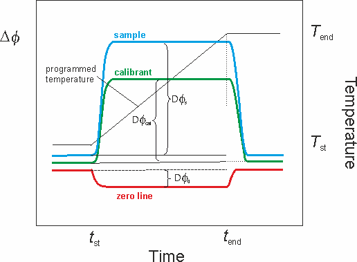
Figure 3. DSC measuring curves for the determination of heat capacities.

 

First, the zero line is recorded using two empty crucibles. Next, a calibrant substance (usually alumina, i.e. synthetic sapphire) is placed in the sample crucible and the temperature program is repeated. Finally, the calibrant is replaced by the sample under study (keeping the crucible) and the temperature program run a third time. The ordinate difference between the traces of the calibrant curve and of the zero line obtained for a given time t leads to the scorresponding value of ε_Φ :

(4)

where Cp (cal) represents the heat capacity of the calibrant. Once the variation of K_Φ with the time and, consequently, with the temperature, is known, the heat capacity of the sample, Cp(cal), can be derived from the difference between the traces of the sample curve and the zero line:

(5)

The samples are enclosed in crucibles, which may or may not be hermetically sealed, and exist in a variety of shapes, depending on the type of apparatus and application. Crucibles are usually made of high thermal conductivity materials and aluminum is by far the most widely used. As illustrated in Figure 2, the reference normally consists of an empty crucible identical to the sample crucible. During the experiments, a purging gas (e.g. helium, argon, nitrogen) is flowed through the cell at a constant rate to ensure that the atmospheric conditions are as uniform as possible in all experiments.

Go to top