Calvet-drop microcalorimeter
The Calvet microcalorimeter (Figure 1) is a heat flow calorimeter. It has most frequently been used in the determination of enthalpies of phase transition (such as vaporization, ΔvapH, and sublimation, ΔsubH) and heat capacities of solids or liquids by the drop method [1-3]. A scheme of the experimental set-up, which requires samples of only 1-5 mg mass, is illustrated in Figure 2.
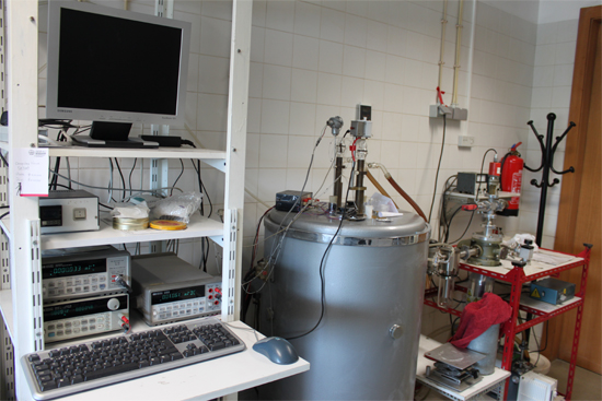
Figure 1. Picture of the Calvet microcalorimeter.
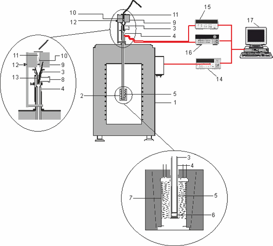
Figure 2. Sheme of the experimental set-up. 1, microcalorimetric elements, 2, glass vessel 3, Teflon tube, 4, brass cylinder, 5, resistance coil for electrical calibration, 6, thermopile, 7, inlet to the vacuum/inert gas line, 8, furnace, 9, sample, 10, miniature platinum resistance sensor, 11, movable pin, 12, guide funnel 13, nanovoltmeter, 14, multimeter, 15, power supply, 16, computer, 17.
The apparatus is based on a DAM Calvet microcalorimeter, 1, which contains two pairs of microcalorimetric elements and can be operated from room temperature to 473 K. Each pair of elements works in the differential mode, with one element used for measurement and the other functioning as reference. The sample cell is inserted into one of the four microcalorimetric elements, 2, and a matching reference cell is inserted into the corresponding twin element, which is placed in opposite position (not seen in the figure). The cell assembly consists of a long tubular glass vessel 3 inserted into a Teflon tube, 4, that terminates in a brass cylinder, 5. The bottom of the glass cell fits tightly into the brass cylinder and sits at the top of piece, 6, supporting a 200 Ω manganin resistance coil used for electrical calibration. The heat flow into or out of the cell is detected with the thermopile, 7, that surrounds the brass cylinder 6 inside the measuring element, 2, of the microcalorimeter. The inlet 8 is connected to a vacuum/inert gas line, which can be used to control the atmosphere inside the cell. The furnace, 9, initially containing the sample, 10, is positioned above the inlet of the glass cell 3. The sample is placed into the central well of the furnace, which is closed at the top by a small lid supporting a miniature platinum resistance sensor, 11, and at the bottom by a movable pin, 12. Pulling this pin back drops the sample, through the guide funnel 13, into the calorimeter. The differential heat flow across the thermopiles of the reference and sample cells is measured as a potential difference, by using an Agilent nanovoltmeter, 14. The electrical calibration circuit consists of the manganin resistance mentioned above connected in a four wire configuration to a multimeter, 15 and a power supply, 16. The data acquisition and the electrical calibration are computer controlled, 17, by using the in house developed CBCAL 1.0 program. The data acquisition and the electrical calibration are computer controlled, 14, by the in-house developed CBCAL 1.0 program.
The general operating procedure can be exemplified for an enthalpy of sublimation measurement. Figure 3 illustrates the sequence of output curves typically obtained in this case.
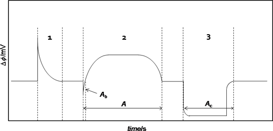
Figure 3. Typical output curve obtained of an experiment.
These correspond to plots of the differential heat flow rate, ΔΦ, between the measuring (S) and reference (R):
 |
(1) |
cells as a function of time, t. After dropping the sample into the calorimetric cell an endothermic peak, 1, due to the heating of the sample from 298 K to the calorimeter temperature T is observed (the area, A, of this curve can be used to calculate the heat capacity of the compound, see below). When the signal returns to the baseline the sample and reference cells are simultaneously evacuated to ~0.13 Pa and the measuring curve, 2, associated with the sublimation of the compound is acquired. The sublimation experiment is followed by an electrical calibration, 3, where a known amount of heat is dissipated inside the cell by Joule effect.
This is achieved by passing a current of intensity I through the resistance coil winded around piece F (Figure 2), during a pre-selected time t. The current is generated as a result of the application of a potential difference V, to the resistance terminals. The calibration constant, ε, is obtained from:
 |
(2) |
where A
 |
(3) |
where m and M are the mass and the molar mass of the sample, respectively, A is the area of the experimental curve, and Ab is the area of the pumping background contribution determined in independent runs where the atmosphere inside the calorimetric cells (normally air or N2) is pumped out by means of the above mentioned vacuum system.
The average specific heat capacity of the sample between T1 and T2 can be calculated from:
 |
(4) |
where A is the area of peak a, T1 is temperature of the furnace I and T2 is the temperature of the calorimetric cell. Heat capacity measurements as a function of the temperature can be performed by, for example, successively changing the initial temperature (T1) of the samples dropped from oven I into the calorimetric cell, kept at constant temperature (T2).