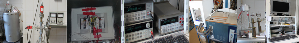
LKB 10700-1 flow microcalorimeter
The flow microcalorimeter currently in use at the Molecular Energetics Group is a modified version of a LKB 10700-1 apparatus [1]. The modifications included the implementation of a computer-controlled data acquisition and handling system and the replacement of the ancillary equipment for pumping, pre-thermostatization, thermopile output measurement, and electrical calibration. The calorimeter is of heat flow type and is suitable for studies involving pure liquids or solutions. It is particularly useful in the determination of enthalpies of mixture, ΔmixH and dilution, ΔdilH [2-4] and in the evaluation of the energetics and kinetics of slow reactions [5]. The apparatus general view and scheme are shown in Figure 2.
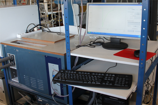
Figure 1. Picture of the LKB 10700-1 flow microcalorimeter.
The apparatus currently in use in the Molecular Energetics Group is a modified version of a LKB 10700-1 flow microcalorimeter, which involved the implementation of a computer-controlled data acquisition and handling system and the entire replacement of the ancillary equipment for pumping, pre-thermostatization, thermopile output measurement and electrical calibration. A general view and a scheme of the apparatus are shown in Figure 2.
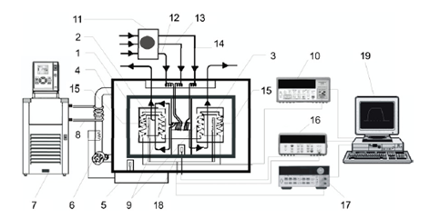
Figure 2. Scheme of the modified LKB 10700-1 flow microcalorimeter apparatus used in this work: (1) calorimeter proper, (2) mixing cell, (3) reference cell, (4) thermostated air jacket, (5) air thermostat, (6) fan, (7) pre-thermostatic bath, (8) cooling coil, (9) thermopiles, (10) nanovoltmeter used to monitor the output of the thermopiles, (11) multi-channel peristaltic pump, (12, 13) tubes leading to the mixing cell, (14) tube leading to the reference cell, (15) electrical resistance used for calibration, (16) multimeter of the calibration circuit, (17) power supply of the calibration circuit, (18) precision thermistor used to measure the temperature of the calorimeter proper, (19) computer for experiment control and data acquisition.
The calorimeter proper, 1, consists of a heat sink containing a pair of calorimetric elements: the measuring cell (mixing cell, 2) and the reference cell (flow-through cell, 3). The calorimeter proper is surrounded by a thermostated air jacket, 4, whose temperature is controlled by means of a LKB 10700-1 air thermostat, 5. Air is circulated inside the jacket by using fan 6. The temperature control of the air jacket also includes a pre-thermostatic bath from which water flows through the cooling coil 8. The differential heat flow across the thermopiles, 9, connecting both cells to the heat sink is measured as a potential difference, by using an Agilent nanovoltmeter, 10. Reagent solutions are simultaneously pumped from storage flasks, using two peristaltic pumps, 11 (see Figure 3 below). Tubes 12 and 13 lead the solutions into the mixing cell, 2, and tube 14 is connected to the flow-through cell, 3. The electrical calibration circuit of the mixing or of the flow-through cells consists of a 50 Ω resistance, 15, embedded in the cell block connected in a four wire configuration to a multimeter, 16, and a power supply, 17. The data acquisition and the electrical calibration are computer controlled, 19, using the in house developed CBCAL 1.0 program.
The two feeding configurations used at the different stages of a dilution experiment are illustrated in Figure 3 for the nicotinic acid (NA) + water (H
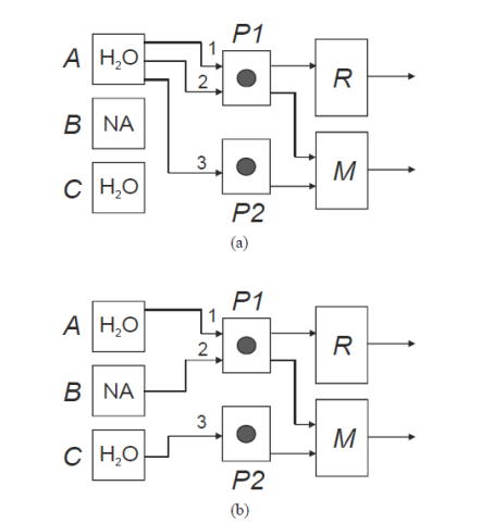
Figure 3. Feeding configurations used at the different stages of a dilution experiment.
The resultant output curve, which corresponds to a plot of the differential heat flow rate, ΔΦ, between the measuring (S) and reference (R):
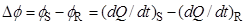 |
(1) |
cells as a function of time, t, is shown in Figure 4.
Figure 4. Typical output curve obtained of an experiment.
Water is initially pumped from storage flask A through three feeding lines: line 1 connected to the flow-through cell which serves as reference, R, and lines 2 and 3 connected to the mixing cell, M (Figure 3a). After definition of a sufficiently long initial baseline (Figure 4, section 1), the dilution process is started by transferring the feeding ends of tubes 2 and 3 into flasks B and C containing the nicotinic acid solution and water, respectively. This causes a progressive shift of the calorimetric signal from the baseline. Once a the amplitude of the shift becomes stable and well defined (S
The final baseline of the dilution stage serves as the initial baseline of the calibration period. At the onset of calibration a constant potential V, is applied to a resistance inside the mixing cell, 2, causing a current of intensity I to flow for a predetermined time interval, t. As a result of the heat dissipated in the resistance a deviation of the measuring curve from the baseline, corresponding to an amplitude S
 |
(2) |
where P is the power dissipated on average by Joule heating inside the cell. The molar enthalpy of the dilution process is derived from:
 |
(3) |
where Se is the deviation of the measuring curve from the baseline during the dilution period, and q